What if free will is not an illusion and can be reconciled with the known laws of physics?

 -by I, Quantum

Table of Contents

Synopsis – Free Will

  1. The Question of Free Will
  2. Dualities
  3. About Quantum Mechanics and Biology
  4. The Origin of Choice and the First/Third Person Duality
  5. Crisscross Entanglement and the Nonlinear Schrödinger Equation
  6. The Mind’s Eye and Free Will
  7. Making Sense of Experimental Results in Neuroscience
  8. What is it like to be an Electron?
  9. Predictability
  10. (stress, meditation, sex, understanding, self-awareness, Gödel’s incompleteness theorem, qualia of the senses, moral responsibility, vice, love, consciousness)

    Powerpoint Summary of What if free will is not an illusion? 


What if the miracle behind evolution is quantum mechanics?

 -by I, Quantum

Table of Contents
  1. Miracles and Monsters
  2. Occam’s Fat-Shattering Razor
  3. Complexity is the Key – in Machine Learning and DNA    
  4. The Protein Folding Problem
  5. The Nature of Quantum Mechanics – Infinite, Non-Local, Computing Capacity
  6. Solving the Quantum Measurement Problem – Pointers, Decoherence, & Quantum Dynamics
  7. Quantum Networks – Using Dynamics to Restore and Extend Entanglement
  8. Quantum Biology – Noisy, Warm, Dynamical Quantum Systems
  9. Quasicrystals & Phasons – Shadows of Life?
  10. Holography & The Ultimate Quantum Network – A Living Organism
  11. Quantum Mechanics and Evolution
  12. Experimental Results in Evolutionary Biology

Images- Left/Top: Drawing Hands by M. C. Escher, 1948, Right/bottom: Mandelbrot set by Reguiieee both via Wikipedia

Evolution – Synopsis

We explore a means, originally suggested by Schrödinger in 1944, by which mutations as quantum transitions of a whole organism may be physically feasible. Like an electron in a hydrogen atom makes a transition to a higher energy state upon absorption of a photon, the organism transitions to a more stable energy state – probably by absorption of a photon in the UV spectrum (chapter VIII). There are several substantial challenges that must be met for this to be physically plausible.

First up, the trouble with quantum theories and evolution is that quantum mechanics does not care about fitness, or survival, it only cares about energy states, e.g. the ground state, or first excited state in the hydrogen atom. We bridge this gap by showing that stress in the environment induces instability in the organism’s energy state. The key is recognizing a.) that entanglement itself plays a role in binding the organism together – something which has been shown to be true in the case of the electron clouds of DNA. But, b.) environmental stress muddles it. Therefore, adapting to stress means a mutation that tends to increase, or at least restore entanglement. This upside bias in entanglement leads to the selective bias toward higher complexity. The quantum transition, which involves tautomerization of nucleotides in DNA via quantum tunneling (C<->A, G<->T) and photon absorption, is thus to a more stable energy configuration (chapter XI).

Second, for a quantum transition to occur, the organism must have the relevant pieces entangled together as One system of molecules (DNA<->RNA<->Proteins). In other words, the proteins in contact with the environment must been entangled with the DNA that encodes them so they function as one system (chapter XI). The marginal stability of proteins – the small energy differences between various configurations – is an essential characteristic too (chapter IV). If true, this empowers the system with the infinite computational power of quantum mechanics (a power illuminated plainly, and computationally modeled by the path integral formulation of quantum mechanics) (chapter V). The quantum calculus of photon absorption, and thereby mutation to the DNA sequence, instantaneously considers all the possible pathways by which the organism might adapt to the stress. The collective sum of these path integrals can be thought of as a sort of hologram. The path chosen is the result of quantum probabilities manifested in a complex holographic interference pattern. This hologram is not in the visual spectrum but in the frequency range relevant to the vibrational, conformational and other states of biomolecules – probably THz among others. It is the coherent tool an organism uses to direct its’ own growth non-locally – like DNA directs its own transcription (chapter X). An analogy is drawn to quasicrystals where vast collective, non-local atomic rearrangements, called phasons, are seen to occur in the laboratory, elucidating quantum mechanical effects on an intermediate scale (chapter IX).

Third, while it is virtually impossible to imagine the sustained static quantum entanglement that scientists pursue in today’s quantum computers in biological systems, i.e. decoherence, biology takes a different tact. Its approach is dynamical, with constant renewed entanglement and constant decoherence (chapter VIII). It is closer, by analogy, to the dynamical environment described in a quantum network where entanglement can be restored and extended over vast distances (chapter VII). Research has shown dynamical entangled quantum systems can exist in environments even when static entanglement is impossible (chapter VIII). This is crucial to life and critical to the miracles of evolution.

Fourth, even with the infinite computational power of quantum mechanics available to the organism, focusing this computational power is critical to leveraging it, just as interference is critical to Shor’s factoring algorithm (chapter V), and for that, life needs to control its own complexity (chapter III). The simplest description of the world is the correct one – the philosophical principle of Occam’s razor (chapter II). This principle forces DNA to keep the blueprint of the organism simple so that the genetic code is modularized, objected oriented, plug-and-play like. This gives the path integrals a fighting chance of finding a working adaptation to environmental stress. But, the relationship is reciprocal. A simple description of the organism is equivalent to a more stable energy state – a key point derived from machine learning (chapter III). A key result of this is that mutations cannot be truly random, they have an element of quantum mechanical uncertainty for sure, but they must be very organized in nature, swapping out one module for another. And this is, indeed, what we see in experiments: organism can change a few nucleotides, delete sections, insert sections, or even make gross genetic rearrangements to adapt to stress with minimal failures (chapter XII). All are allowed quantum transitions with various probabilities given by the mathematics of quantum mechanics of complex dynamical systems- as described in the solution to the quantum measurement problem (chapter VI). This high degree of ordered simplicity combined with quantum computational power is the secret of the miraculous leaps that occur in evolutionary pathways (chapter XI).

Last, this description of biological systems allows us to draw an analogy between some very personal, first person experiences and the fundamental quantum mechanical nature of the universe. For instance, “love” is naturally affiliated with “Oneness”, or becoming “One” with others – like quantum entanglement is to particles. “Understanding” is also a fundamental defining trait of the human experience, yet life is utilizing this principle in DNA – manifest in its simplicity – from life’s very beginning. And, “creativity”, something that we as humans take such pride in, appears as the result of the infinite quantum computational power of the universe at the level of basic particles. Creative capacity grows as organisms, and the entanglement therein, grows more complex – it doesn’t suddenly appear. In higher-level organisms the range of creativity transitions from just the space of biomolecules and DNA to the external space of human endeavor (via the brain), but this is still all creativity nonetheless. A picture irresistibly emerges that these three traits, “love”, “understanding”, and “creativity” aren’t random accidental traits selected for the during “X billion years of evolution” at all, but defining characteristics of the quantum mechanical universe all the way from humans, to single-cell life, to sub-cellular life, to fundamental particles. It is a picture in which natural selection plays a role, but in which life is a cooperative, not a cutthroat competition. Indeed, the metaphor that life is the Universe trying to understand itself is apropos (chapter XII).

What if the Miracle Behind Evolution is Quantum Mechanics?


(CC BY-NC 4.0)

I, Quantum

“…about forty years ago the Dutchman de Vries discovered that in the offspring even of thoroughly pure-bred stocks, a very small number of individuals, say two or three in tens of thousands, turn up with small but ‘jump-like’ changes, the expression ‘jump-like’ not meaning that the change is so very considerable, but that there is a discontinuity inasmuch as there are no intermediate forms between the unchanged and the few changed. De Vries called that a mutation. The significant fact is the discontinuity. It reminds a physicist of quantum theory – no intermediate energies occurring between two neighbouring energy levels. He would be inclined to call de Vries’s mutation theory, figuratively, the quantum theory of biology. We shall see later that this is much more than figurative. The mutations are actually due to quantum jumps in the gene molecule. But quantum theory was but two years old when de Vries first published his discovery, in 1902. Small wonder that it took another generation to discover the intimate connection!” – Erwin Schrödinger, ‘What is Life?‘ (1944)

Table of Contents

    1. Miracles and Monsters
    2. Occam’s Fat-Shattering Razor
    3. Complexity is the Key – in Machine Learning and DNA    
    4. The Protein Folding Problem
    5. The Nature of Quantum Mechanics – Infinite, Non-Local, Computing Capacity
    6. Solving the Quantum Measurement Problem – Pointers, Decoherence, & Quantum Dynamics
    7. Quantum Networks – Using Dynamics to Restore and Extend Entanglement
    8. Quantum Biology – Noisy, Warm, Dynamical Quantum Systems
    9. Quasicrystals & Phasons – Shadows of Life?
    10. Holography & The Ultimate Quantum Network – A Living Organism
    11. Quantum Mechanics and Evolution
    12. Experimental Results in Evolutionary Biology

Synopsis

I. Miracles and Monsters

What is going on with life? It is utterly amazing all the things these plants and creatures of mother nature do! Their beauty! Their complexity! Their diversity! Their ability to sustain themselves! The symbiotic relationships! Where did it all come from? If evolution is the right idea, how does it work? We’re not talking about the little changes, the gradual changes proposed by Charles Darwin. We understand there is natural selection going on, like pepper colored moths and Darwin’s finches. We’re talking about the big changes – the evolutionary leaps apparently due to mutations affecting gene expression, a process known as saltation. How do these mutations know what will work – shouldn’t there be a bunch of failed abominations everywhere from the gene mutations that screwed up? Shouldn’t a mix up be far more likely than an improvement? Is it possible mutations are adaptive as Jean-Baptiste Lamarck, a predecessor of Darwin, originally proposed? That is, could it be that the environment, rather than random changes, is the primary driver of adaptation?


Imagine selecting architectural plans on a two-story house. Suppose we randomly pick from the existing set of millions of blueprints for the upstairs, and separately pick the plans for the downstairs and put them together. How many times would you expect this house to be functional? The plumbing and electrical systems to work? Suppose we start with a blueprint for a house and then select randomly the plans for just the living room and swap that into the original? What are the chances this would produce a final blue print that was workable? Seemingly very small we should say! We expect there should be all these monstrous houses, with leaking plumbing, short circuited electricity, windows looking out at walls, doorways to nowhere, and grotesque in style!


Turns out Evolutionary Biologists have been concerned with this problem for a long time. A geneticist named Richard Goldschmidt was the first scientist to coin the term “hopeful monster” in 1933 in reference to these abominations. Goldschmidt’s theory was received with skepticism. Biologists argued: if evolution did produce big changes in a species then how would these mutants find a mate? For most of the 20th century Goldschmidt’s ideas were on the back burner, scientists were focused on gradualism as they uncovered many examples of gradual evolutionary changes in nature, supporting the natural selection hypothesis. But, recent scientific results reveal the environment does, indeed, have a deep impact on the traits of offspring. The adaptations of embryos in experiments are an example:


“The past twenty years have vindicated Goldschmidt to some degree. With the discovery of the importance of regulatory genes, we realize that he was ahead of his time in focusing on the importance of a few genes controlling big changes in the organisms, not small-scales changes in the entire genome as neo-Darwinians thought. In addition, the hopeful monster problem is not so insurmountable after all. Embryology has shown that if you affect an entire population of developing embryos with a stress (such as a heat shock) it can cause many embryos to go through the same new pathway of embryonic development, and then they all become hopeful monsters when they reach reproductive age.” – Donald R. Prothero in his book Evolution: What the Fossils Say and Why it Matters (2007); via rationalwiki.org.

These discoveries prompted Evolutionary Biologist Olivia Judson to write a wonderful article “The Monster is Back, and it’s Hopeful.” (via Wikipedia) Still, we are left wondering: where are all the hopeless monsters? All the embryos either adapt to the stress or keep the status quo – there are no failures. Shouldn’t some suffer crippling mutations? Are epigenetic factors involved? And, perhaps most importantly, even with environmental feedback, how do organisms know how to adapt – i.e. how is the process of adaptation so successful?


The puzzle would not be complete, however, without also considering some amazing leaps that have occurred along the tree of life, for example, the mutations that lead to the evolution of the eye. How does life figure out it can construct this extended precisely shaped object – the eyeball – and set up the lens, the muscles to focus it, the photoreceptors and the visual cortex to make sense of the image? It seems like we would need a global plan, a blueprint of an eye, before we start construction! Not only that, but to figure it out independently at least fifty-times-over in different evolutionary branches? Or, how did cells make the leap from RNA to DNA, as is widely believed to be the case, in the early evolution of single celled organisms? Evolutionary biologists puzzle that to make that leap life would need to know the DNA solution would work before it tried it. How should life be so bold – messing with the basic gene structure would seem fraught with danger? How could life know? And, don’t forget, perhaps the most amazing leap of all, where does this amazing human intelligence come from? We humans, who are probing the origins of the Universe, inventing or discovering mathematics, building quantum computers and artificial intelligence, and seeking to understand our very own origin– however it may have happened – how did WE come to be?


To frame the problem, let’s talk classical statistics for a second and consider the following situation: suppose we have 100 buckets into which we close our eyes and randomly toss 100 ping pong balls. Any that miss we toss again. When we open our eyes, what distribution should we expect? All in a single cup? Probably not. Scattered over many cups with some cups holding more ball than others? Probably something like that. If we repeat this experiment zillions of times, however, sooner or later, we will find one instance with them all in the same bucket. Is this a miracle? No, of course not. Once in a while amazingly unlikely things do happen. If we tossed the balls repeatedly and each time all landed in the same bucket, now that would feel like a miracle! That’s what’s weird about life – the miracles seem to keep happening again and again along the evolutionary tree. The ping pong balls appear to bounce lucky for Mother Nature!

II. Occam’s Fat-Shattering Razor

The Intelligent Design folks ardently point out the miraculous nature of life despite being labeled as pseudoscientists by the scientific community at large. However, no can one deny that the amazing order we see in biological systems does have the feel of some sort of intelligent design, scientifically true or not. The trouble is that these folks postulate an Intelligent Designer is behind all these miracles. In fact, it is possible that they are correct, but, there is a problem with this kind of hypothesis: it can be used to explain anything! If we ask “how did plants come to use photosynthesis as a source of energy?” we answer: “the Designer designed it that way”. And, if we ask “how did the eye come to exist in so many animal species?”, again, we can only get “the Designer designed it that way”. The essential problem is that this class of hypotheses has infinite complexity.

“It may seem natural to think that, to understand a complex system, one must construct a model incorporating everything that one knows about the system. However sensible this procedure may seem, in biology it has repeatedly turned out to be a sterile exercise. There are two snags with it. The first is that one finishes up with a model so complicated that one cannot understand it: the point of a model is to simplify, not to confuse. The second is that if one constructs a sufficiently complex model one can make it do anything one likes by fiddling with the parameters: a model that can predict anything predicts nothing.” – John Maynard Smith and Eörs Szathmáry (Hat tip Gregory Chaitin)

The field of learning theory forms the foundation of machine learning. It contains the secret sauce that is behind many of the amazing artificial intelligence applications today. This list includes achieving image recognition on par with humans, self-driving cars, Jeopardy! champion Watson, and the amazing 9-dan Go program AlphaGo [see Figure 2]. These achievements shocked people all over the world – how far and how fast artificial intelligence had advanced. Half of this secret sauce is a sound mathematical understanding of complexity in computer models (a.k.a. hypotheses) and how to measure it. In effect learning theory has quantified the philosophical principal of Occam’s razor which says that the simplest explanation is the correct one – we can now measure the complexity of explanations. Early discoveries in the 1970’s produced the concept of the VC dimension (also known as the “fat-shattering” dimension) named for its discoverers, Vladimir Vapnik and Alexey Chervonenkis. This property of a hypothesis class measures the number of observations that it is guaranteed to be able to explain. Recall a polynomial with, say, 11 parameters, such as:

P(x)=c_0+c_1x^1+c_2x^2+c_3x^3+c_4x^4+c_5x^5+c_6x^6+c_7x^7+c_8x^8+c_9x^9+c_{10}x^{10}

can be fit to any 11 data points [see Figure 1]. This function is said to have a VC dimension of 11. Don’t expect this function to find any underlying patterns in the data though! When a function with this level of complexity is fit to an equal number of data points it is likely to over-fit. The key to having a hypothesis generalize well, that is, make predictions that are likely to be correct, is having it explain a much greater number of observations than its complexity.


Figure 1: Noisy (roughly linear) data is fitted to both linear and polynomial functions. Although the polynomial function is a perfect fit, the linear version can be expected to generalize better. In other words, if the two functions were used to extrapolate the data beyond the fit data, the linear function would make better predictions. Image and caption by Ghiles [CC BY-SA 4.0] on Wikimedia.

Nowadays measures of complexity have become much more acute: the technique of margin-maximization in support vector machines, regularization in neural networks and others have had the effect of reducing the effective explanatory power of a hypothesis class, thereby limiting its complexity, and causing the model to make better predictions. Still, the principal is the same: the key to a hypothesis making accurate predictions is about managing its complexity relative to explaining known observations. This principal applies whether we are trying to learn how to recognize handwritten digits, how to recognize faces, how to play Go, how to drive a car, or how to identify “beautiful” works of art. Further, it applies to all mathematical models that learn inductively, that is, via examples, whether machine or biological. When a model fits the data with a reasonable complexity relative to the number of observations then we are confident it will generalize well. The model has come to “understand” the data in a sense.


Figure 2: The game of Go. The AI application AlphaGo defeated one of the best human Go players, Lee Sedol, 4 games to 1 in March,2016 by Goban1 via Wikimedia Commons.

The hypothesis of Intelligent Design, simply put, has infinite VC dimension, and, therefore can be expected to have no predictive power, and that is what we see – unless, of course, we can query the Designer J! But, before we jump on Darwin’s bandwagon we need to face a very grim fact: the hypothesis class characterized by “we must have learned that during X billion years of evolution” also has the capacity to explain just about anything! Just think of the zillions of times this has been referenced, almost axiom-like, in the journals of scientific research!

III. Complexity is the Key – In Machine Learning and DNA

As early as 1945 a computational device known as a neural network (a.k.a. a multi-layered perceptron network) was invented. It was patterned after the networks formed by neuron cells in animal brains [see figure 3]. In 1975 a technique called backpropagation was developed that significantly advanced the learning capability of these networks. They were “trained” on a sample of input data (observations), then could be used to make predictions about future and/or out-of-sample data.


Neurons in the first layer were connected by “synaptic weights” to the data inputs. The inputs could be any number of things, e.g. one pixel in an image, the status of a square on a chessboard, or financial data of a company. These neurons would multiply the input values by the synaptic weights and sum them. If the sum exceeded some threshold value the neuron would fire and take on a value of 1 for neurons in the second layer, otherwise it would not fire and produce a value of 0. Neurons in the second layer were connected to the first via another set of synaptic weights and would fire by the same rules, and so on to the 3rd, 4th, layers etc. until culminating in an output layer. Training examples were fed to the model one at a time. The network’s outputs were compared against the known results to evaluate errors. These were used to adjust the weights in the network via the aforementioned backpropagation technique: weights that contributed to the error were reduced while weights contributing to a correct answer were increased. With each example, the network followed the error gradient downhill (gradient descent). The training stopped when no further improvements were made.


Figure 3: A hypothetical neural network with an input layer, 1 hidden layer, and an output layer, by Glosser.ca (CC BY-SA) via Wikimedia Commons.

Neural Networks exploded onto the scene in the 1980’s and stunned us with how well they would learn. More than that, they had a “life-like” feel as we could watch the network improve with each additional training sample, then become stuck for several iterations. Suddenly the proverbial “lightbulb would go on” and the network would begin improving again. We could literally watch the weights change as the network learned. In 1984 the movie “The Terminator” was released featuring a fearsome and intelligent cyborg character, played by Arnold Schwarzenegger, with a neural network for a brain. It was sent back from the future where a computerized defense network, Skynet, had “got smart” and virtually annihilated all humanity!

The hysteria did not last, however. The trouble was that while neural networks did well on certain problems, on others they failed miserably. Also, they would converge to a locally optimal solution but often not a global one. There they would remain stuck only with random perturbations as a way out – a generally hopeless proposition in a difficult problem. Even when they did well learning the in-sample training set data, they would sometimes generalize poorly. It was not understood why neural nets succeeded at times and failed at others.

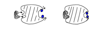
In the 1990’s significant progress was made understanding the mathematics of the model complexity of neural networks and other computer models and the field of learning theory really emerged. It was realized that most of the challenging problems were highly non-linear, having many minima, and any gradient descent type approach would be vulnerable to becoming stuck in one. So, a new kind of computer model was developed called the support vector machine. This model rendered the learning problem as a convex optimization problem – so that it had only one minima and a globally optimal result could always be found. There were two keys to the support vector machine’s success: first it did something called margin-maximization which reduced overfitting, and, second, it allowed computer scientists to use their familiarity with the problem to choose an appropriate kernel – a function which mapped the data from the input feature space into a smooth, convex space. Like a smooth bowl-shaped valley, one could follow the gradient downhill to a global solution. It was a way of introducing domain knowledge into the model to reduce the amount of twisting and turning the machine had to do to fit the data. Bayesian techniques offered a similar helping hand by allowing their designers to incorporate a “guess”, called the prior, of what the model parameters might look like. If the machine only needed to tweak this guess a little bit to come up with a posterior, the model could be interpreted as a simple correction to the prior. If it had to make large changes, that was a complex model, and, would negatively impact expected generalization ability – in a quantifiable way. This latter point was the second half of the secret sauce of machine learning – allowing clever people to incorporate as much domain knowledge as possible into the problem so the learning task was rendered as simple as possible for the machine. Simpler tasks required less contortion on the part of the machine and resulted in models with lower complexity. SVM’s, as they became known, along with Bayesian approaches were all the rage and quickly established machine learning records for predictive accuracy on standard datasets. Indeed, the mantra of machine learning was: “have the computer solve the simplest problem possible”.


Figure 4: A kernel, , maps data from an input space, where it is difficult to find a function that correctly classifies the red and blue dots, to a feature space where they are easily separable – from StackOverflow.com.

It would not take long before the science of controlling complexity set in with the neural net folks – and the success in learning that came with it. They took the complexity concepts back to the drawing board with neural networks and came out with a new and greatly improved model called a convolutional neural network. It was like the earlier neural nets but had specialized kinds of hidden layers known as convolutional and pooling layers (among others). Convolutional layers significantly reduced the complexity of the network by limiting neurons connectivity to only a nearby region of inputs, called the “receptive field”, while also capturing symmetries in data – like translational invariance. For example, a vertical line in the upper right hand corner of the visual field is still a vertical line if it lies in the lower left corner. The pooling layer neurons could perform functions like “max pooling” on their receptive fields. They simplified the network in the sense that they would only pass along the most likely result downstream to subsequent layers. For example, if one neuron fires, weakly indicating a possible vertical line, but, another neuron fires strongly indicating a definite corner, then only the latter information is passed onto the next layer of the network [see Figure 5].


Figure 5: Illustration of the function of max pooling neurons in a pooling layer of a convolutional neural network. By Aphex34 [CC BY-SA 4.0] via Wikimedia Commons

The idea for this structure came from studies of the visual cortex of cats and monkeys. As such, convolutional neural networks were extremely successful at enabling machines to recognize images. They quickly established many records on standardized datasets for image recognition and to this day continue to be the dominant model of choice for this kind of task. Computer vision is on par with human object recognition ability when the human subject is given a limited amount of time to recognize the image. A mystery that was never solved was: how did the visual cortex figure out its own structure.

Interestingly, however, when it comes to more difficult images, humans can perform something called top-down reasoning which computers cannot replicate. Sometimes humans will look at an image, not recognize it immediately, then start using a confluence of contextual information and more to think about what the image might be. When ample time is given for humans to exploit this capability we exhibit superior image recognition capability. Just think back to the last time we were requested to type in a string of disguised characters to validate that we were, indeed, human! This is the basis for CAPTCHA: Completely Automated Public Turing test to tell Computers and Humans Apart. [see Figure 6].


Figure 6: An example of a reCAPTCHA challenge from 2007, containing the words “following finding”. The waviness and horizontal stroke were added to increase the difficulty of breaking the CAPTCHA with a computer program. Image and caption by B Maurer at Wikipedia

While machine learning was focused on quantifying and managing the complexity of models for learning, the dual concept of the Kolmogorov complexity had already been developed in 1965 in the field of information theory. The idea was to find the shortest description possible of a string of data. So, if we generate a random number by selecting digits at random without end, we might get something like this:

5.549135834587334303374615345173953462379773633128928793.6846590704…

and so on to infinity. An infinite string of digits generated in this manner cannot be abbreviated. That is, there is no simpler description of the number than an infinitely long string. The number is said to have infinite Kolmogorov complexity, and is analogous to a machine learning model with infinite VC dimension. On the other hand, another similar looking number, , extends out to infinity:

3.14159265358979323846264338327950288419716939937510582097494459230…

never terminating and never repeating, yet, it can be expressed in a much more compact form. For example, we can write a very simple program to perform a series approximation of to arbitrary accuracy using the Madhava-Leibniz series (from Wikipedia):


So, has a very small Kolmogorov complexity, or minimum description length (MDL). This example illustrates the abstract, and far-from-obvious nature of complexity. But, also, illustrates a point about understanding: when we understand something, we can describe it in simple terms. We can break it down. The formula, while very compact, acts as a blueprint for constructing a meaningful, infinitely long number. Mathematicians understand . Similar examples of massive data compression abound, and some, like the Mandelbrot set, may seem biologically inspired [see Figure 7].

Figure 7: This image illustrates part of the Mandelbrot set (fractal). Simply storing the 24-bit color of each pixel in this image would require 1.62 million bits, but a small computer program can reproduce these 1.62 million bits using the definition of the Mandelbrot set and the coordinates of the corners of the image. Thus, the Kolmogorov complexity of the raw file encoding this bitmap is much less than 1.62 million bits in any pragmatic model of computation. Image and caption By Reguiieee via Wikimedia Commons

Perhaps life, though, has managed to solve the ultimate demonstration of MDL – the DNA molecule itself! Indeed, this molecule, some 3 billion nucleotides (C, A, G, or T) long in humans, encodes an organism of some 3 billion-billion-billion (3 \times 10^{26} \colon 1  ) amino acids. A compression of about a billion-billion to 1 (1 \times 10^{18} \colon 1  ). Even including possible epigenetic factors as sources of additional blueprint information (epigenetic tags are thought to affect about 1% of genes in mammals), the amount of compression is mind boggling. John von Neuman pioneered an algorithmic view of DNA, like this, in 1948 in his work on cellular automata. Biologists know, for instance, that the nucleotide sequences: “TAG”, “TAA”, and “TGA” act as stop codons (Hat tip Douglas Hoftstadter in Gödel, Escher, Bach: An Eternal Golden Braid) in DNA and signal the end of a protein sequence. More recently, the field of Evolutionary Developmental Biology (a.k.a. evo-devo) has encouraged this view:

The field is characterized by some key concepts, which took biologists by surprise. One is deep homology, the finding that dissimilar organs such as the eyes of insects, vertebrates and cephalopod mollusks, long thought to have evolved separately, are controlled by similar genes such as pax-6, from the evo-devo gene toolkit. These genes are ancient, being highly conserved among phyla; they generate the patterns in time and space which shape the embryo, and ultimately form the body plan of the organism. Another is that species do not differ much in their structural genes, such as those coding for enzymes; what does differ is the way that gene expression is regulated by the toolkit genes. These genes are reused, unchanged, many times in different parts of the embryo and at different stages of development, forming a complex cascade of control, switching other regulatory genes as well as structural genes on and off in a precise pattern. This multiple pleiotropic reuse explains why these genes are highly conserved, as any change would have many adverse consequences which natural selection would oppose.

New morphological features and ultimately new species are produced by variations in the toolkit, either when genes are expressed in a new pattern, or when toolkit genes acquire additional functions. Another possibility is the Neo-Lamarckian theory that epigenetic changes are later consolidated at gene level, something that may have been important early in the history of multicellular life.” – from Wikipedia

Inspired by von Neuman and the developments of evo-devo, Gregory Chaitin in 2010 published a paper entitled “To a Mathematical Theory of Evolution and Biological Creativity“. Chaitin characterized DNA as a software program. He built a toy-model of evolution where computer algorithms would compute the busy beaver problem of mathematics. In this problem, he tries to get the computer program to generate the biggest integer it can. Like children competitively yelling out larger and larger numbers: “I’m a million times stronger than you! Well, I’m a billion times stronger. No, I’m a billion, billion times. That’s nothing, I’m a billion to the billionth power times stronger!” – we get the idea. Simple as that. The program has no concept of infinity and so that’s off limits. There is a subroutine that randomly “mutates” the code at each generation. If the mutated code computes a bigger integer, it becomes the de facto code, otherwise it is thrown out (natural selection). Lots of times the mutated code just doesn’t work, or it enters a loop that never halts. So, an oracle is needed to supervise the development of the fledgling algorithms. It is a very interesting first look at DNA as an ancient programming language and an evolving algorithm. See his book, Proving Darwin: Making Biology Mathematical, for more.


Figure 8: Graph of variation in estimated genome sizes in base pairs (bp). Graph and caption by Abizar at Wikipedia

One thing is for certain: the incredible compactness of DNA molecules implies it has learned an enormous amount of information about the construction of biological organisms. Physicist Richard Feynman famously said “what I cannot create, I do not understand.” Inferring from Feynman: since DNA can create life (maybe “build” is a better word), it therefore understands it. This is certainly part of the miracle of biological evolution – understanding the impact of genetic changes on the organism. The simple description of the organism embedded in DNA allows life to predictably estimate the consequences of genetic changes – it is the key to generalizing well. It is why adaptive mutations are so successful. It is why the hopeless monsters are missing! When embryos adapt to stress so successfully, it’s because life knows what it is doing. The information is embedded in the genetic code!


Figure 9: Video of an Octopus camouflaging itself. A dramatic demonstration of how DNA understands how to build organisms – it gives the Octopus this amazing toolkit! Turns out it has an MDL of only 3 basic textures and the chromatophores come in only 3 basic colors! – by SciFri with marine biologist Roger Hanlon

In terms of house blueprints, it means life is so well ordered that living “houses” are all modular. The rooms have such symmetry to them that the plumbing always goes in the same corner, the electrical wiring always lines up, the windows and doors work, even though the “houses” are incredibly complex! You can swap out the upstairs, replace it with the plans from another and everything will work. Change living rooms if you want, it will all work, total plug-and-play modular design. It is all because of this remarkably organized, simple MDL blueprint.


The trouble is: how did this understanding come to be in the first place? And, even understanding what mutations might successfully lead to adaptation to a stress, how does life initiate and coordinate the change among the billions of impacted molecules throughout the organism? Half of the secret sauce of machine learning was quantifying complexity and the other half was allowing creative intelligent beings, such as ourselves, to inject our domain knowledge into the learning algorithm. DNA should have no such benefit, or should it? Not only that, but recent evidence suggests the role of epigenetic factors, such as methylation of DNA, is significant in heredity. How does DNA understand the impact of methylation? Where is this information stored? Seemingly not in the DNA, but if not, then where?

IV. The Protein Folding Problem

“Perhaps the most remarkable features of the molecule are its complexity and its lack of symmetry. The arrangement seems to be almost totally lacking in the kind of regularities which one instinctively anticipates, and it is more complicated than has been predicated by any theory of protein structure. Though the detailed principles of construction do not yet emerge, we may hope that they will do so at a later stage of the analysis.” – John Kendrew et al. upon seeing the structure of the protein myoglobin under an electron microscope for the first time, via “The Protein Folding Problem, 50 Years On” by Ken Dill

DNA exists in every cell in every living organism. Not only is it some 3 billion nucleotides long, but it encodes 33,000 genes which express over 1 million proteins. There are several kinds of processes that ‘repeat’ or copy the nucleotides sequences in DNA:

1.) DNA is replicated into additional DNA for cell division (mitosis)

2.) DNA is transcribed into RNA for transport outside the nucleus

3.) RNA is translated into protein molecules in the cytoplasm of the cell – by NobelPrize.org

Furthermore, RNA does not only play a role in protein synthesis. Many types of RNA are catalytic – they act like enzymes to help reactions proceed faster. Also, many other types of RNA play complex regulatory roles in cells (see this for more: the central dogma of molecular biology).

Genes act as recipes for protein molecules. Proteins are long chains of amino acids that become biologically active only after they fold. While often depicted as messy squiggly strands lacking any symmetry, they ultimately fold very specifically into beautifully organized highly complex 3-dimensional shapes such as micro pumps, bi-pedaled walkers called kinesins, whip-like flagella that propel the cell, enzymes and other micro-machinery. The proteins that are created ultimately determine the function of the cell.


Figure 10: This TEDx video by Ken Dill gives an excellent introduction to the protein folding problem and shows the amazing dynamical forms these proteins take.

The protein folding problem has been one of the great puzzles in science for 50 years. The questions it poses are:

  1. “How does the amino acid sequence influence the folding to form a 3-D structure?
  2. There are a nearly infinite number of ways a protein can fold, how can proteins fold to the correct structure so fast (nanoseconds for some)?
  3. Can we simulate proteins with computers?”
    – from The Protein-Folding Problem, 50 Years On by Ken Dill

Nowadays scientists understand a great number of proteins, but several questions remain unanswered. For example, Anfinsen’s dogma is the postulate that the amino acid sequence alone determines the folded structure of the protein – we do not know if this is true. We also know that molecular chaperones help other proteins to fold, but are thought not to influence the protein’s final folded structure. We can produce computer simulations of how proteins fold. However, this is only possible in special cases of simple proteins where there is an energy gradient leading the protein downhill to a global configuration of minimal energy [see figure 11]. Even in these cases, the simulations do not accurately predict protein stabilities or thermodynamic properties.

Figure 11: This graph shows the energy landscape for some proteins. When the landscape is reasonably smoothly downhill like this, protein folding can be simulated. Graph By Thomas Splettstoesser (www.scistyle.com) via Wikimedia Commons


Figure 12: A TED Video (short) by David Bolinsky showing the complexity of the protein micro-machinery working away inside the cell. Despite all this complexity, organization, and beauty, little is understood about how proteins fold to form these amazing machines.

Protein folding generally happens in a fraction of a second (nanoseconds in some cases), which is mind boggling given the number of ways it could fold. This is known as Levinthal’s paradox, posited in 1969:

“To put this in perspective, a relatively small protein of only 100 amino acids can take some 10^{100}   different configurations. If it tried these shapes at the rate of 100 billion a second, it would take longer than the age of the universe to find the correct one. Just how these molecules do the job in nanoseconds, nobody knows.” – Technology Review.com, “Physicists discover quantum law of protein folding”    

The Arrhenius equation is used to estimate chemical reaction rates as a function of temperature. Turns out the application of this equation to protein folding misses badly. In 2011, L. Luo and J. Lu published a paper entitled “Temperature Dependence of Protein Folding Deduced from Quantum Transition“. They show that quantum mechanics can be used to correctly predict the proper temperature dependence of protein folding rates (hat tip chemistry.stackexchange.com). Further, globular proteins (not the structural or enzymatic kind) are known to be marginally stable, meaning that there is very little energy difference between the folded, native state, and the unfolded state. This kind of energy landscape may open the door to a host of quantum properties.     

V. The Nature of Quantum Mechanics – Infinite, Non-Local, Computing Capacity

“It is impossible that the same thing belong and not belong to the same thing at the same time and in the same respect.”; “No one can believe that the same thing can (at the same time) be and not be.”; “The most certain of all basic principles is that contradictory propositions are not true simultaneously.” – Aristotle’s Law of Non-Contradiction, “Metaphysics (circa 350 B.C.) Via Wikipedia

Max Planck in 1900, in order to solve the blackbody radiation problem, and Albert Einstein in 1905, to explain the photoelectric effect, postulated that light itself was made of individual “energy quanta” and so began the theory of quantum mechanics. In the early 20th century many titans of physics would contribute to this strange theory, but a rare, rather intuitive, discovery occurred in 1948 when Richard Feynman invented a tool called the path integral. When physicists wanted to calculate the probability that, say, an electron, travels from A to B they used the path integral. The path integral appears as a complex exponential function like e^{-i\Phi(x)} in physics equations, but this can be conceptually understood simply as a two-dimensional wave because:

e^{-i\Phi(x)}=cos\Phi(x)+isin\Phi(x)

The real component represents one direction (e.g. horizontal-axis), while the other, “imaginary”, component another (e.g. vertical-axis). This complex function in the path integral, and in quantum mechanics in general, just means the wave is two-dimensional, not one. Think of a rope with one person holding each end. A vertical flick by one person sends a vertical wave propagating along the rope toward the other – this is not the path integral of quantum mechanics. Neither is a horizontal flick. Instead, imagine making a twisting flick, both vertical and horizontal. A corkscrew shaped wave propagates down the rope. This two-dimensional wave captures the nature of quantum mechanics and the path integral, but the wave is not known to be something physical like the wave on the rope. It is, rather, a wave of probability (a.k.a. a quantum wave function).


Figure 13: The titans of quantum physics -1927 Solvay Conference on Quantum Mechanics by Benjamin Couprie via Wikimedia Commons.

The path integral formulation of quantum mechanics is mathematically equivalent to the Schrödinger equation – it’s just another way of formulating the same physics. The idea for the electron is to sum (integrate) over all the possible ways it can go from A to B, summing all the 2-D waves together (a.k.a. amplitudes). To get the right answer – the one that agrees with experiment – we must also consider very exotic paths. The tools that help us do this are Feynman diagrams which illustrate all the particle physics interactions allowed along the way. So, a wave propagates from A to B via every possible path it can take in space and time and at every point therein it considers all the allowed Feynman diagrams (great intro to Feynman diagrams here). The more vertices there are in the diagram the smaller that particular diagram’s contribution – each additional vertex adds a probability factor of about 1/137th. The frequency and wavelength of the waves change with the action (a function of the energy of the particle). At B, all the amplitudes from every path are summed, some interfering constructively, some destructively, and the resultant amplitude squared is the probability of the electron going from A to B. But, going from A to B is not the only thing that path integrals are good for. If we want to calculate the probability that A scatters off of B then interacts with C, or A emits or absorbs B, the cross-section of A interacting with D, or whatever, the path integral is the tool to do the calculation. For more information on path integrals see these introductory yet advanced gold-standard lectures by Feynman on Quantum Electro-Dynamics: part 1, 2, 3 and 4.


Figure 14: In this Feynman diagram, an electron and a positron
annihilate
, producing a photon (represented by the blue sine wave) that becomes a quark
antiquark pair, after which the antiquark radiates a gluon (represented by the green helix). Note: the arrows are not the direction of motion of the particle, they represent the flow of electric charge. Time always moves forward from left to right. Image and caption by Joel Holdsworth [GFDL, CC-BY-SA-3.0], via Wikimedia Commons


Path integrals apply to every photon of light, every particle, every atom, every molecule, every system of molecules, everywhere, all the time, in the observable universe. All the known forces of nature appear in the path integral with the peculiar sometimes exception of gravity. Constant, instantaneous, non-local, wave-like calculations of infinitely many possibilities interfering all at once is the nature of this universe when we look really closely at it. The computing power of the tiniest subsets are infinite. So, when we fire a photon, an electron, or even bucky-balls (molecules of 60 carbon atoms!) for that matter, at a two-slit interferometer, on the other side we will see an interference pattern. Even if fired one at a time, the universe will sum infinitely many amplitudes and a statistical pattern will slowly emerge that reveals the wave-like interference effects. The larger the projectile the shorter it’s wavelength. The path integrals still must be summed over all the round-about paths, but the ones that are indirect tend to cancel out (destructively interfere) making the
interference pattern much more narrow. Hence, interference effects are undetectable in something as large as a baseball, but still theoretically there.


Figure 15: Results from the Double slit experiment: Pattern from a single slit vs. a double slit.By Jordgette [CC BY-SA 3.0 ] via Wikimedia Commons

Feynman was the first to see the enormous potential in tapping into the infinite computing power of the universe. He said, back in 1981:

“We can’t even hope to describe the state of a few hundred qubits in terms of classical bits. Might a computer that operates on qubits rather than bits (a quantum computer) be able to perform tasks that are beyond the capability of any conceivable classical computer?” – Richard Feynman [Hat tip John Preskill]

Quantum computers are here now and they do use qubits instead of bits. The difference is that, while a classical 5-bit computer can be in only one state at any given time, such as “01001”, a 5-qubit quantum computer can be in all possible 5-qubit states (2^5 ) at once: “00000”, “00001”, “00010”, “00011”, …, “11111”. Each state, k, has a coefficient, \alpha_k , that, when squared, indicates the probability the computer will be in that state when we measure it. An 80-qubit quantum computer can be in 2^{80} states at once – more than the number of atoms in the observable universe!

The key to unlocking the quantum computer‘s power involves two strange traits of quantum mechanics: quantum superposition and quantum entanglement. Each qubit can be placed into a superposition of states, so it can be both “0” and “1” at the same time. Then, it can be entangled with other qubits. When two or more qubits become entangled they act as “one system” of qubits. Two qubits can then be in four states at once, three qubits in eight, four qubits in 16 and so on. This is what enables the quantum computer to be in so many states at the same time. This letter from Schrödinger to Einstein in 1935 sums it up:

“Another way of expressing the peculiar situation is: the best possible knowledge of a whole does not necessarily include the best possible knowledge of its parts…I would not call that one but rather the characteristic trait of quantum mechanics, the one that enforces its entire departure from classical lines of thought…” – Erwin Schrödinger, Proceedings of the Cambridge Philosophical Society, submitted Aug 14, 1935. [Hat tip to John Preskill]

We can imagine starting a 5-qubit system in the ground state, all qubits initialized to “0”. The computer is in the state “00000”, no different than a classical computer so far. With the first tick of the clock (less than a nanosecond), we can place the 1st qubit into a superposition of states, state 1 = “00000” and state 2 = “10000”, with coefficients \alpha_1  and \alpha_2 indicating the probability of finding the system in each state respectively upon measurement. Now we have, in a sense, two computers operating at once. On the 2nd tick of the clock, we place the 2nd bit into a superposition too. Now our computer is in four states at once: “00000”, “10000”, “01000”, and “11000” with probabilities \alpha_1 , \alpha_2 , \alpha_3 , and \alpha_4 , respectively. And so on. In a handful of nanoseconds our computer could be in thirty-two states at once. If we had more qubits to work with, there is no theoretical limit to how many states the quantum computer can be in at once. Other quantum operations allow us to entangle two or more qubits in any number of ways. For example, we can entangle qubit #1 and qubit #2 such that if qubit #1 has the value of “0”, then qubit #2 must be “1”. Or, we can entangle qubits #3, #4, and #5 so that they must all have the same value: all zeros, “000”, or all ones, “111” (an entanglement known as a GHZ state). Once the qubits of the system are entangled, the states of the system can be made to interfere with each other, conceptually like the interference in the two-slit experiment. The right quantum algorithm of constructive and destructive interference unleashes the universe’s infinite quantum computational power.


In 1994 Peter Shor invented an algorithm, known as Shor’s algorithm (a tutorial is here), for factorizing integers on a quantum computer. Factorizing is a really hard problem and that’s why this approach is used to encrypt substantially all of the information we send over the internet (RSApublic key cryptography). For example, the problem of factoring a 500-digit integer takes 10^{12} CPU years on a conventional computer – longer than the age of the universe. A quantum computer with the same clock speed (a reasonable assumption), would take two seconds! [Hat tip to John Preskill for the stats] Factoring of integers is at least in a class of problems known to be NP, and more than likely NP-Hard, in its computational complexity. That means the calculation time on a conventional computer grows exponentially bigger, proportional to e^N , as the size of the integer, N, grows (actually, this is only a conjecture, not proven, see P=NP? for more). On a quantum computer, the calculation time only grows logarithmically, proportional to (log N)^3 . That is a HUGE difference! That means, for instance, that quantum computers will trivially break all current public key encryption schemes! All the traffic on the internet will be visible to anyone that has access to a quantum computer! And still, quantum algorithms and quantum computing are very much in their infancy. We have a long way to go before we understand and can harness the full potential of quantum computing power!


Figure 16: Quantum subroutine for order finding in Shor’s algorithm by Bender2k14 [CC BY-SA 4.0], via Wikimedia Commons. Based on Figure 1 in Circuit for Shor’s algorithm using 2n+3 qubits by Stephane Beauregard.


There are many ways to implement a quantum computer. It is possible to make qubits out of electron-spins, so, say the spin is pointing up, that would represent a value of “1”, and down, a value of “0”. Electrons can never have any spin but either up or down, i.e. they’re quantized, but, they can exist in a superposition of both. They can also be entangled together. Other implementations involve photons, nuclear spins, configurations of atoms (called topological qubits), ion traps, and more. While there are many different approaches, and still a lot to learn, all of today’s approaches do have something in common: they try to isolate the qubits in a very cold (near absolute zero), dark, noiseless, vibration free, static environment. Nothing is allowed to interact with the qubits, nor are new qubits allowed to be added or removed during the quantum computation. We have a fraction of a second to finish the program and measure the qubits before decoherence sets in and all quantum information in the qubits is lost to the environment. Researchers are constantly trying to find more stable qubits that will resist decoherence for longer periods. Indeed, there is no criterion that says a quantum computer must be digital at all – it could be an analog style quantum computer and do away with qubits altogether.

IBM has a 5-qubit quantum computer online right now that anyone can access. They have online tutorials that teach how to use it too. The best way for us to develop an intuition for quantum mechanics is to get our hands dirty and write some quantum programs, called “quantum scores” – like a musical score. It really is not hard to learn, just counter-intuitive at first. Soon, intuition for this kind of programming will develop and it will feel natural.

Another company, D-Wave, is working on an alternative approach to quantum computing called quantum annealing. A quantum annealer does not allow us to write quantum programs, instead it is specifically designed to find global solutions (a global minimum) to specific kinds of mathematical optimization problems (here is tutorial from D-Wave). This process takes advantage of yet another strange property of quantum mechanics called quantum tunneling. Quantum tunneling allows the computer to tunnel from one local minimum to another, in a superposition of many different paths at once, until a global minimum is found. While they do have a 1,000+qubit commercial quantum annealer available, some physicists remain skeptical of D-Wave’s results.

VI. Solving the Quantum Measurement Problem – Pointers, Decoherence & Quantum Dynamics

Despite all the incredible practical success with quantum technology there was still an incompleteness about quantum’s interpretation. The trouble had to do with reconciling the quantum world with the macroscopic classical world. It wasn’t just a matter of a different set of equations. Logic itself was different. John Bell proved this when he published what became known as Bell’s inequality (1964). He came up with a simple equation, essentially:

N(A,~B)+N(B,~C) \geq  N(A,~C)

This video by Leonard Susskind explains it best – “the number of things in A and not B plus the number of things in B and not C is greater than or equal to the number of things in A and not C”. It’s easy to visualize with Venn diagrams and straight forward to prove this mathematically, just like a theorem of set theory. It involves no physical assumptions, just pure mathematics. But, turns out quantum mechanics doesn’t obey it! (see also Hardy’s paradox (1992)
for a really good brain teaser)

The trouble with quantum mechanics is that classical logic does not apply because the quantum world does not have the property of realism. Realism means that the things around us exist independently of whether we observe them. If there are mathematical sets A, B, and C those sets exist independent of the mathematician. In the quantum world, if we observe set A, it can change set B and C. The order that we observe the sets matters too. Realism means the proverbial tree that falls in the forest makes a sound whether we hear it or not. In the quantum world that’s not true. The tree exists in a superposition of states both making and not making a sound until someone, or something, observes it. This does not sound like a very plausible description of our practical experience though. From early on we all learn that nobody really disappears when we play “peek-a-boo”! It’s almost axiomatic. Realism does seem to be a property of the macroscopic universe. So, what gives?

The most common interpretation of quantum mechanics was called the Copenhagen interpretation. It said that the wave function would “collapse” upon measurement per the Born rule. It was a successful theory in that it worked – we could accurately predict what the results of a measurement would be. Still, this was kind of a band-aid on an otherwise elegant theory and the idea of having two entirely different logical views of the world was unsettling. Some physicists dissented and argued that it was not the responsibility of physicists to interpret the world, it was enough to have the equations to make predictions. This paradox became known as the quantum measurement problem and was one of the great unsolved mysteries of physics for over one hundred years. In the 1970’s the theory of decoherence was developed. This helped physicists understand why it was hard to keep things entangled, in a superposition, but it didn’t solve the problem of how things transitioned to a definite state upon measurement – it only partially addressed the problem. In fact, many brilliant physicists gave up on the idea of one Universe – to them it would take an infinite spectrum of constantly branching parallel Universes to understand quantum mechanics. This was known as the many world’s interpretation.


Figure 17: Excellent video introduction to quantum entanglement by Ron Garret entitled “The Quantum Conspiracy: What popularizers of QM Don’t Want You to Know“. Garret’s argument is that measurement “is” entanglement. We now understand entanglement is the first step in the measurement process, followed by asymptotic convergence to pointer states of the apparatus.

In 2013 A. Allahverdyan, R. Balian, and T. Nieuwenhuizen published a ground-breaking paper entitled “Understanding quantum measurement from the solution of dynamical models“. In this paper the authors showed that the measurement problem can be understood within the context of quantum statistical mechanics alone – pure quantum mechanics and statistics. No outside assumptions, no wave function collapse. All smooth, time reversible, unitary evolution of the wave function. The authors show that when a particle interacts with a macroscopic measuring device, in this case an ideal Curie-Weiss magnet, it first entangles with the billion-billion-billon (~10^{27}  ) atoms in the device momentarily creating a vast superposition of states. Then, two extreme cases are examined: first, if the coupling to the measuring device is much stronger than the coupling to the environment, the system cascades asymptotically to a pointer state of the device. This gives the appearance of wave-function collapse, but it is not that, it is a smooth convergence, maybe like a lens focusing light to a single point. This is the case when the number of atoms, which all have magnetic moments, in the measuring device is large. At first this seems a counter-intuitive result. One might expect the entanglement to keep spreading throughout and into the environment in an increasingly chaotic and complex way, but this does not happen. The mathematics prove it.

In the second extreme, when the coupling to the environment is much stronger, the system experiences decoherence – the case when the number of atoms in the measuring device is small. This happens before entanglement can cascade to a pointer state and so the system fails to register a measurement.

The author’s results are applied to a particle’s spin interacting with a particular measuring device, but the results appear completely general. In other words, it may be that measurements in general, like the cloud chamber photos of particle physics or the images of molecular spectroscopy, are just asymptotic pointer states – no more wave-particle duality, just wave functions. Just more or less localized wave functions. It means that the whole of the classical world may just be an asymptotic state of the much more complex quantum world. Measurement happens often because pointer states are abundant, so the convergence gives the illusion of realism. And, in the vast majority of cases, this approximation works great. Definitely don’t stop playing “peek-a-boo”!

It may turn out that biological systems occupy a middle ground between these two extremes – many weak couplings but not so many strong ones. Lots of densely packed quantum states, but a distinct absence of pointers. In such a system, superpositions could potentially be preserved for longer time scales because it may be that the rate of growth of entanglement propagating through the system may equal the rate of decoherence. It may even be that no individual particle remains entangled but a dynamic wave of entanglement – an entanglement envelope – followed by a wave of decoherence will describe the quantum dynamics. A dynamic situation where entanglement is permanent, but always on the move.


VII. Quantum Networks – Using Dynamics to Restore and Extend Entanglement

Quantum networks use a continual dynamical sequence of entanglement to teleport a quantum state for purposes of communication. It works like this: suppose A, B, C, & D are qubits and we entangle A with B in one location, and C with D in another (most
laboratory quantum networks have used entangled photons from an EPR source for qubits). The two locations are 200km apart. Suppose the farthest we can send B or C without losing their quantum information to decoherence is 100km. So, we send B and C to a quantum repeater halfway in between. At the repeater station B and C are entangled (by performing a Bell state measurement, e.g. passing B and C thru a partially transparent mirror). Instantaneously, A and D will become entangled! Even if some decoherence sets in with B and C, when they interact at the repeater station full entanglement is restored. After that it does not matter what happens to B or C. They may remain entangled, be measured, or completely decohere – A and D will remain entangled 200km apart! This process can be repeated with N quantum repeaters to connect arbitrarily far away locations and to continually restore entanglement. It can also be applied in a multiple party setting (3 or more network endpoints). We could potentially have a vast number of locations entangled together at a distance – a whole quantum internet! When we are ready to teleport a quantum state, \left|\phi\right> , (which could be any number of qubits, for instance) over the network, we entangle \left|\phi\right> with A in the first location and then D will instantaneously be entangled in a superposition of states at the second location – one of which will be the state \left|\phi\right> ! In a multi-party setting, every endpoint of network receives the state \left|\phi\right> instantaneously! Classical bits of information must be sent from A to D to tell which one of the superposition is the intended state. This classical communication prevents information from traveling faster than the speed of light – as required by Einstein‘s special theory of relativity.


Figure 18: A diagram of a quantum network from Centre for Quantum Computation & Communication Technology. EPR sources at either end are sources of entangled qubits where A&B and C&D are entangled. The joint measurement of B & C occurs at the quantum repeater in the middle entangling A & D at a distance.

Researchers further demonstrated experimentally that macroscopic atomic systems can be entangled (and a quantum network established) by transfer of light (the EM field) between the two systems (“Quantum teleportation between light and matter” – J. Sherson et al., 2006). In this case the atomic system was a spin-polarized gas sample of a thousand-billion (10^{12} ) cesium atoms at room temperature and the distance over which they were entangled was about \frac{1}{2} meter.


VIII. Quantum Biology – Noisy, Warm, Dynamical Quantum Systems

Quantum Biology is a field that has come out of nowhere to be at the forefront of pioneering science. But 20 years ago, virtually no one thought quantum mechanics had anything to do with biological organisms. On the scale of living things quantum effects just didn’t matter. Nowadays quantum effects seem to appear all over biological systems. The book “Life on the Edge: The Coming Age of Quantum Biology” by J. McFadden and J. Al-Khalili (2014) is a New York Times bestseller and gives a great comprehensive introduction. Another, slightly more technical introduction, is this paper “Quantum physics meets biology” by M. Ardnt, T. Juffmann, and V. Vedral (2009), and more recently this paper
Quantum biology” (2013) by N. Lambert et al. A summary of the major research follows:

Photosynthesis: Photosynthesis represents probably the most well studied of quantum biological phenomenon. The FMO complex (Fenna-Mathews-Olsen) of green-sulphur bacteria is a large complex making it readily accessible. Light-harvesting antennae in plants and certain bacteria absorb photons creating an electronic excitation. This excitation travels to a reaction center where it is converted to chemical energy. It is an amazing reaction achieving near 100% efficiency – nearly every single photon makes its way to the reaction center with virtually no energy wasted as heat. Also, it is an ultrafast reaction taking only about 100 femtoseconds. Quantum coherence was observed for the first time in “Evidence for wavelike energy transfer through quantum coherence in photosynthetic systems” by Engel et al. (2007). The energy transfer seems to involve quantum exciton
delocalization that is assisted by quantum phonon states and environmental noise. It is believed that coherent interference may guide the excitations to the reaction centers. This paper proves unequivocally that photosynthesis uses quantum processes – something that there is surprisingly strong resistance to by classicists.

Enzyme Catalysis:
Enzymes catalyze reactions speeding up reactions rates by enormous amounts. Classical factors can only explain a small fraction of this. Quantum tunneling of hydrogen seems to play an important role. Enzymes are vibrating all the time and it is unclear what role coherence and superposition effects may also contribute to reaction rate speed-ups.

Avian Compass: Several bird species, including robins and pigeons, are believed to use quantum radical-pair production to sense the Earth’s magnetic field for migratory purposes (the avian compass). Pair production involves the protein cryptochrome and resides in the bird’s eye.

Olfactory sense: Traditional theories of olfaction describe a “lock & key” method where molecules (the key) are detected if they fit into a specific geometric configuration (the lock). We have about 400 differently shaped smell receptors, but recognize 100,000 different smells. For example, the human nose can distinguish ferrocene and nickelocene which both have similar geometry. It has been proposed that the olfactory sense uses quantum electron tunneling to detect the vibrational spectra of molecules.

Vision receptors: One of the key proteins involved in animal vision is called retinal. The retinal molecule undergoes conformational change upon absorption of a photon. This allows humans to detect even just a handful of emitted photons. The protein rhodopsin, active in octopi in the dark ocean depths, may be able to detect single photons.

Consciousness: R. Penrose was the first to propose that quantum mechanics had a role in consciousness in his book “The Emperor’s New Mind” (1989). Together with S. Hameroff, he developed a theory known as Orch-OR (orchestrated objective reduction) which has received much attention. While the theory remains highly controversial, it has been instrumental in jump starting research into possible relationships between quantum mechanics and consciousness. The compelling notion behind this has to do with quantum’s departure from determinism – a.k.a. the “annihilation operator” of freewill, i.e. quantum probabilities could potentially allow freewill to enter the picture. Generally, the thinking is that wave function collapse has something to do with conscious choice. The conversation about consciousness is a deeply fascinating subject unto itself and we will address this in a subsequent supposition.

Mutation: In 1953, shortly after discovering DNA, J. Watson and F. Crick proposed that mutation may occur through a process called tautomerization. The DNA sequence is comprised of nucleotides: cytosine, adenine, guanine and thymine. The only difference between guanine and thymine is the location of a hydrogen atom in the molecular structure. Tautomerization is a process by which the hydrogen atom quantum tunnels through the molecular structure to allow guanine to transform into thymine, and similarly adenine into cytosine. Only recently have quantum simulations become sophisticated enough to test this hypothesis. This paper “UV-Induced Proton Transfer between DNA Strands” by Y. Zhang et al. (2015) shows experimental evidence that ultraviolet (UV) photons can induce tautomerization. This is a very important mechanism we will return into later.

Even with the growth and success of quantum biology, and the advances in sustaining quantum entanglement (e.g. 10 billion ions entangled for 39 minutes at room temperature – 2013), some scientists look at the warm, wet environment of living organisms and conclude there is no way “to keep decoherence at bay” in such an environment. Such arguments are formidable in the context of static quantum systems – like those used for developing present day quantum computers. But, biological systems tend to be dynamical, operating far from thermal equilibrium, with lots of noise and many accessible quantum rotational, vibrational, torsional and quasiparticle states. Moreover, we have discussed the importance of managing complexity in machine learning (chapter II and III), science has had a lot of success with classical molecular chemistry (balls and sticks), and, classical calculations are much simpler than quantum calculations. Shouldn’t we cling to this simpler approach until it is utterly falsified? Maybe so, but while quantum mechanical calculations are certainly more computationally intensive, they may not be more complex as a theory. More importantly, classical science is simply struggling to correctly predict observed results all over biological systems. A thorough study of quantum biological processes is deservedly well underway.

In 2009 J. Cai, S. Popescu, and H. Briegel published a paper entitled “Dynamic entanglement in oscillating molecules and potential biological implications” (follow-up enhancements in 2012 are here) which has shown that entanglement can continually recur in biological molecules in a hot noisy environment in which no static entanglement can survive. Conformational change is ubiquitous in biological systems – this is the shape changing that many proteins rely on to function. Conformational change induced by noisy, thermal energy in the environment repetitively pushes two sites of the bio-molecule together entangling them. When the two sites come together, they “measure” each other. That means that their spins must either line up together, or be opposite. The system will sit in a superposition of both, with each spin dependent upon the other, i.e. entangled, during at least a portion of the oscillation cycle. If the conformational recurrence time is less than the decoherence time, entanglement may be preserved indefinitely. Entanglement can be continually restored even in the presence of very intense noise. Even when all entanglement is temporarily lost, it will be restored cyclically. We wonder if there were not only two sites, but a string of sites, could a wave of entanglement spread, via this method, throughout the system? Followed by a wave of decoherence. In such a circumstance, perhaps an “envelope” of entanglement might cascade through the system (as we discussed in chapter VI). Such a question could be addressed in the context of quantum dynamical models as in the solution to the quantum measurement problem.


Figure 19: “Conformational changes of a bio-molecule, induced, for example, by the interaction with some other chemical, can lead to a time-dependent interaction between different sites (blue) of the molecule.” – from “Dynamic entanglement in oscillating molecules and potential biological implications” by J. Cai, S. Popescu, and H. Briegel (2009)

IX. Quasicrystals & Phasons – Shadows of Life?

“A small molecule might be called ‘the germ of a solid’. Starting from such a small solid germ, there seem to be two different ways of building up larger and larger associations. One is the comparatively dull way of repeating the same structure in three directions again and again. That is the way followed in a growing crystal. Once the periodicity is established, there is no definite limit to the size of the aggregate. The other way is that of building up a more and more extended aggregate without the dull device of repetition. That is the case of the more and more complicated organic molecule in which every atom, and every group of atoms, plays an individual role, not entirely equivalent to that of many others (as is the case in a periodic structure). We might quite properly call that an aperiodic crystal or solid and express our hypothesis by saying: ‘We believe a gene – or perhaps the whole chromosome fibre’ – to be an aperiodic solid.” – Erwin Schrödinger, What is Life? (1944) chapter entitled ‘The Aperiodic Solid’

Crystals are structures that derive their unique properties (optical transparency, strength, etc.) from the tight packing, symmetric structure of the atoms that comprise them – like quartz, ice, or diamonds. There are only so many ways atoms can be packed together in a periodic pattern to form a two-dimensional crystal: rectangles and parallelograms (i.e. 2-fold symmetry), triangles (3-fold), squares (4-fold), or hexagons like snowflakes or honeycombs (6-fold). These shapes can be connected tightly to one another leaving no gaps in between. Moreover, there is no limit on how extensive crystals can be since attaching more atoms is just a matter of repeating the pattern. Mathematically, we can tessellate an infinite plane with these shapes. Other shapes, like pentagons, don’t work. There are always gaps. In fact, mathematicians have proven no other symmetries are allowed in crystals! These symmetries were “forbidden” in nature and crystallographers never expected to see them. But, in 1982, Dan Shechtman did! When studying the structure of a lab-created alloy of aluminum and manganese (Al_6Mn ) using an electron microscope, he saw a 5-fold symmetric diffraction pattern (Bragg Diffraction) [see Figure 20]. Most crystallographers were skeptical. Shechtman spent two years scrutinizing his work, and, after ruling out all other possible explanations, published his findings in 1984. Turns out, what he discovered was a quasicrystal. In 2011 he was awarded the Nobel Prize in chemistry for his discovery.


Figure 20: Electron diffraction pattern of an icosahedral Zn-Mg-Ho quasicrystal by Materialscientist (Own work) [CC BY-SA 3.0 or GFDL], via Wikimedia Commons

Quasicrystals were not supposed to exist in nature because they were thought to require long-range forces to develop. The forces that were thought to guide atomic assembly of crystals, electromagnetic Coulomb forces, are dominated by local (nearest neighbor) interactions. Still, today, we can make dozens of different quasicrystals in the lab, and, they have been found a handful of times in nature. Physicists have postulated that the non-local effects of quantum mechanics are involved and this is what enables quasicrystals to exist.


Figure 21: Example of 5-fold symmetry may be indicative of biological quasicrystals. (First) flower depicting 5-fold symmetry from “Lotsa Splainin’ 2 Do”, (second) plant with 5-fold symmetric spiral from www.digitalsynopsis.com, (third) starfish from www.quora.com, (last) Leonardo Da Vinci’s “The Vitruvian Man” (1485) via Wikipeida

There is evidence of quasicrystals in biological systems as well: protein locations in the bovine papilloma virus appear to show dodecahedral symmetry [see figure 22], the Boerdijk-Coxeter helix (which forms the core of collagen) packs extremely densely and is proposed to have a quasicrystalline structure, pentameric symmetry of neurotransmitters may be indicative of quasicrystals, and general five-fold symmetries in nature [see figure 21] may also be indicative of their presence. Also, the golden ratio which appears frequently in biological systems is implicit in quasicrystal geometry.


Figure 22: Protein locations in a capsid of bovine papilloma virus. (a) Experimental protein density map. (b) Superimposition of the protein density map with a dodecahedral tessellation of the sphere. (c) The idealized quasilattice of protein density maxima. Kosnetsova, O.V.  Rochal, S.B.  Lorman, V.L. “Quasicrystalline Order and Dodecahedron Geometry in Exceptional Family of Viruses“, Phys. Rev. Lett., Jan. 2012, Hat tip to Prescribed Evolution.

Aperiodic tilings give a mathematical description of quasicrystals. We can trace the history of such tilings back to Johannes Kepler in the 1600’s. The most well-known examples are Penrose tilings [see figure 23], discovered by Roger Penrose in 1974. Penrose worked out that a 2-D infinite plane could, indeed, be perfectly tessellated in a non-periodic way -first, using six different shapes, and later with only two. Even knowing what two shapes to use, it is not easy to construct a tiling that will cover the entire plane (a perfect Penrose tile). More likely is that an arrangement will be chosen that will lead to an incomplete tiling with gaps [see figure 23]. For example, in certain two-tile systems, only 7 of 54 combinations at each vertex will lead to a successful quasicrystal. Selected randomly, the chance of successfully building a quasicrystal quickly goes to zero as the number of vertices grows. Still, it has been shown that in certain cases it is possible to construct Penrose tiles with only local rules (e.g. see “Growing Perfect Quasicrystals“, Onoda et al., 1988). However, this is not possible in all cases, e.g. quasicrystals that implement a one-dimensional Fibonacci sequence.


Figure 23: (Left) A failed Penrose tiling. (Right) A successful Penrose tiling. Both are from Paul Steinhardt’s Introduction to Quasicrystals here.

Phasons are a kind of dynamic structural macro-rearrangement of particles. Like phonons they are a quasiparticle. Several particles in the quasicrystal can simultaneously restructure themselves to phase out of one arrangement and into another [see Figure 24-right]. This paper from 2009 entitled “A phason disordered two-dimensional quantum antiferromagnet” studied a theoretical quasicrystal of ultracold atomic gases in optical lattices after undergoing phason distortions. The authors show that delocalized quantum effects grow stronger with the level of disorder in the quasicrystal. One can see how phason-flips disorder the perfect quasicrystaline pattern [see Figure 24-left].

Figure 24: (Left) The difference between an ordered and disordered quasicrystal after several phason-flips from “A phason disorder two-dimension quantum antiferromagnet” by A. Szallas and A. Jagannathan. (Right) HBS tilings of d-AlCoNi (a) boat upright (b) boat flipped. Atomic positions are indicated as Al¼white, Co¼blue, Ni¼black. Large/small circles indicate vertical position. Tile edge length is 6.5A˚. Caption and image from “Discussion of phasons in quasicrystals and their dynamics” by M. Widom.


Figure 25: Physical examples of quasicrystals created in the lab. Both are from Paul Steinhardt’sIntroduction to Quasicrystals“.

In 2015 K. Edagawa et al. captured video via electron microscopy of a quasicrystal, Al_{70.8}Ni_{19.7}Co_{9.5} , growing. They published their observations here: “Experimental Observation of Quasicrystal Growth“. This write-up, “Viewpoint: Watching Quasicrystals Grow” by J. Jaszczak, provides an excellent summary of Edagawa’s findings and we will follow it here: certain quasicrystals, like this one, produce one-dimensional Fibonacci chains. A Fibonacci chain can be generated by starting with the sequence “WN” (W for wide, N for narrow referring to layers of the quasicrystal) and then use the following substitution rules: replace “W” with “WN” and replace “N” with “‘W”. Applying the substitutions one time transforms “WN” into “WNW”. Subsequent application expands the Fibonacci sequence: “WNWWN”, “WNWWNWNW”, “WNWWNWNWWNWWN”, and so on. The continued expansion of the sequence cannot be done without knowledge of the whole one-dimensional chain. Turns out that when new layers of atoms are added to the quasicrystal, they are usually added incorrectly leaving numerous gaps [see Figure 26]. This creates “phason-strain” in the quasicrystal. There may be, in fact, several erroneous layers added before the atoms undergo a “phason-flip” into a correct arrangement with no gaps.

Figure 26:
Portion of an ideal Penrose tiling illustrating part of a Fibonacci sequence of wide (W) and narrow (N) rows of tiles (green). The W and N layers are separated by rows of other tiles (light blue) that have edges perpendicular to the average orientation of the tiling’s growth front. The N layers have pinch points (red dots) where the separator layers touch, whereas the W layers keep the divider layers fully separated. An ideal tiling would require the next layer to be W as the growth front advances. However, Edagawa and colleagues observed a system in which the newly grown layer would sometimes start as an N layer, until a temperature-dependent time later upon which it would transition through tile flipping to become a W layer. (graph and caption are from Jaszczak, J.A. APS Physics)

How does nature do this? Non-local quantum mechanical effects may be the answer. Is the quasicrystal momentarily entangled together so that it not only may be determined what sort of layer, N or W, goes next, but also, so that the action of several atoms may be coordinated together in one coordinated phason-flip?

One cannot help but wonder, does quantum mechanics understand the Fibonacci sequence? In other words, has it figured out that it could start with “WN” and then follow the two simple substitution rules outlined above? This would represent a rather simple description (MDL) of the quasicrystal. And, if so, where does this understanding reside, i.e. where is the quasicrystal’s DNA? Suffice it to say, it has, at the very least, figured out something equivalent. In other words, whether it has understood the Fibonacci sequence or not, whether it has understood the substitution rules or not, it has developed the equivalent to an understanding as it can extend the sequence! So, even if quantum mechanics did not keep some sort of log, or blueprint of how to construct the Fibonacci quasicrystal, it certainly has the information to do so!

X. Holography & The Ultimate Quantum Network – A Living Organism

DNA is a remarkable molecule. Not just because it contains the whole genetic blueprint of the organism distilled in such a simple manner, but also because it can vibrate, rotate, and excite in so many ways. DNA is not natively static. It’s vibrating at superfast frequencies (like nanoseconds and femtoseconds)! Where does all this vibrational energy come from? One would think this energy would dissipate into the surrounding environment. Also puzzling is: why is there a full copy of DNA in every single cell? Isn’t that overkill? This paper, “Is it possible to predict electromagnetic resonances in proteins, DNA and RNA?” by I. Cosic, D. Cosic, and K. Lazar (2016), shows the incredible range of resonant frequencies in DNA. And, not only that, they also show that there is substantial overlap with other biomolecules like proteins and RNA. Perhaps DNA has some deeper purpose. Is it possible DNA is some sort of quantum repeater (chapter VII)? To do so, DNA would need to provide a source of entangled particles (like the EPR photon source in a laboratory quantum network).

This paper “Quantum entanglement between the electron clouds of nucleic acids in DNA” (2010) by E. Rieper, J. Anders, and V. Vedral has shown that entanglement between the electron clouds of neighboring nucleotides plays a critical role in holding DNA together. They oscillate, like springs, between the nucleotides, and occupy a superposition of states: to balance each other out laterally, and to synchronize oscillations (harmonics) along the chain. The former prevents lateral strain on the molecule, and the latter is more rhythmically stable. Both kinds of superpositions exist because they stabilize and lower the overall energy configuration of the molecule! The entanglement is in its ground state at biological temperatures so the molecule will remain entangled even in thermal equilibrium. Furthermore, because the electron clouds act like spacers between the planar nucleotides they are coupled to their vibrations (phonons). If the electron clouds are in a superposition of states, then the phonons will be also.


Figure 27: The structure of the DNA double helix. The atoms in the structure are colour-coded by element and the detailed structure of two base pairs (nucleotides) are shown in the bottom right. The nucleotides are planar molecules primarily aligned perpendicular to the direction of the helix. From Wikipedia.

So, DNA’s electron clouds could provide the entanglement, but where does the energy come from? It could, for instance, come from the absorption of ultraviolet light (UV radiation). While we’re all mindful of the harmful aspect of UV radiation, DNA is actually able to dissipate this energy superfast and super efficiently 99.9% of the time. When DNA does absorb UV radiation, the absorption has been shown to be spread out non-locally along the nucleotide chain and follows a process known as internal conversion where it is thought to be thermalized (i.e. turned into heat). Could UV photons be down-converted and then radiated as photons at THz frequencies instead? One UV photon has the energy to make a thousand THz photons, for instance. We have seen such highly efficient and coherent quantum conversions of energy before in photosynthesis (chapter VIII). Could this be a way of connecting the quantum network via the overlapping resonant frequencies to neighboring DNA, RNA, and proteins? The photons would need to be coherent to entangle the network. Also, we can’t always count on UV radiation, e.g. at night or indoors. If this is to work, there must be another source of energy driving the vibrations of DNA also.

A paper published in 2013 by A. Bolan et al. showed experimental evidence that THz radiation affected the expression of genes in the stem cells of mice suggesting that the THz spectrum is particularly important for gene expression. Phonon modes have been observed in DNA for some time, but not under physiological conditions (e.g. in the presence of water) until now. This paper entitled “Observation of coherent delocalized phonon-like modes in DNA under physiological conditions” (2016) by M. González-Jiménez, et al. gives experimental evidence of coherent quantum phonons states even in the presence of water. These phonons span the length of the DNA sequence, expand and contract the distance between nucleotides, and are thought to play a role in breaking the hydrogen bonds that connect the two DNA strands. They are in the THz regime and allow the strands to open forming a transcription bubble which enables access to the nucleotide sequence for replication. This is sometimes referred to as “DNA breathing“. Hence, it’s plausible these phonon modes can control gene expression, and, possibly exist in a complex superposition with the other states of the DNA molecule. They also are coherent which is critical for extending the quantum network, but, is there any evidence proteins could be entangled too?

In 2015 I. Lundholm, et al. published this paper “Terahertz radiation induces non-thermal structural changes associated with Fröhlich condensation in a protein crystal” showing that they could create something called a Fröhlich condensate when they exposed a collection of protein molecules to a THz laser. Herbert Fröhlich proposed the idea back in 1968 and since then it has been the subject of much debate. Now, finally, we have direct evidence these states can be induced in biological systems. These condensates are special because they involve a macroscopic collection of molecules condensing into a single non-local quantum state that only exists under the right conditions. There are many ways a Fröhlich condensate can form, but, in this case, it involves compression of the atomic helical structure of the proteins. Upon compression, the electrons of millions of proteins in crystalline form align and form a collective vibrational state, oscillating together coherently. This conformational change in the protein is critical to controlling its functioning – something generally true of proteins, e.g. as in enzyme catalysis, and protein-protein interactions (hat tip here for the examples). In the laboratory, the condensate state will last micro- to milli- seconds after exposure to the THz radiation, a long time in biomolecular timescales. Of course, that’s upon exposure to a THz laser. Could DNA THz photon emissions perform the same feat and carry the coherent information on from DNA and entangle proteins in the quantum network as well? Could a whole quantum network involving DNA, RNA, and a vast slew of proteins throughout the organism be entangled together via continuous coherent interaction with the EM field (at THz and other frequencies)? If so, it would give the organism an identity as “One” thing, and, it would connect the proteins which are interacting with the environment with the DNA that encodes them. This would open a possible connection between the tautomerization mutation mechanism (chapter VIII) and environmental stress! In other words, a method by which mutations are adaptive would be feasible, and not just that, but a method which could use quantum computational power to determine how to adapt!

But, then there is the question of energy. Where does the continual energy supply come from to support this network and can it supply it without disrupting coherence? In this paper, “Fröhlich Systems in Cellular Physiology” by F. Šrobár (2012), the author describes the details of a pumping source providing energy to the Fröhlich condensate via ATP, or GTP-producing mitochondria. Could the organism’s own metabolism be the sustaining energy source behind the organism’s coherent quantum network?

In the presence of so much coherence, is it possible dynamical interference patterns, using the EM field, could be directed very precisely by the organism – very much like a hologram? Not a visual hologram but rather, images in the EM field relevant to controlling biomolecular processes (e.g. the KHz, MHz, GHz, and THz domains)? A hologram is a 3-D image captured on a 2-D surface using a laser. The holographic plate is special in that it not only records brightness and color, but also the phase of incident coherent light. When the same frequency of coherent light is shined upon it, it reproduces the 3-D image through interference. The surface does not need to be a 2-D sheet, however. Coherently vibrating systems of molecules throughout the organism could create the interference. Not only that, but if the biological quantum network is in a superposition of many states at once, could it conceivably create a superposition of multiple interference patterns in the 3-D EM field at many different frequencies simultaneously (e.g. 20 MHz, 100 GHz, 1 THz, etc.)? With these interference effects, perhaps the organism directly controls, for instance, microtubule growth in specific regions as shown in this paper “Live visualizations of single isolated tubulin protein self-assembly via tunneling current: effect of electromagnetic pumping during spontaneous growth of microtubule” (2014) by S. Sahu, S. Ghosh, D. Fujita, and A. Bandyopadhyay? The paper shows that when the EM field is turned on, at a frequency that coincides with mechanical vibrational frequency of the tubulin protein molecule, the microtubules may be induced to grow, or, stop growing if the EM field is turned off. Microtubules are structural proteins that help form the cytoskeleton of all cells throughout the organism. Perhaps, more generally, organisms use holographic like interference effects to induce or halt growth, induce conformational changes (with the right frequency), manipulate Fröhlich effects, and generally control protein function throughout themselves? Indeed, it may not only be the case of “DNA directing its own transcription” as many biologists believe, but the organism as One whole directing many aspects of its own development.


Figure 28: (Left) Two photographs of a single hologram taken from different viewpoints, via Wikipedia. (Right) Rainbow hologram showing the change in colour in the vertical direction via Wikipedia.

This process would be more analogous to the growth of a quasicrystal (chapter IX) than a bunch of individual molecules trying to find their way. In the process of growth, mistakes along the way happen, such as misfolded proteins. Because quantum mechanics is probabilistic, some mistakes are inevitable. They become like the phason-strain in the quasicrystal – the quantum network corrects the arrangement through non-local phason-shifts, directed holographically. Rearrangement is not like reallocating balls and sticks as in classical molecular chemistry, but more like phasing out of one configuration of quantum wave functions and into another. Perhaps the quantum computing power of vast superpositions through holographic interference effects, not unlike Shor’s algorithm (chapter V), is the key to solving the highly non-linear, probably NP-hard problems, of organic growth.

Construction of the eye, a process requiring global spatial information and coordination, could be envisioned holographically by the quantum organism in the same way that quantum mechanics understood the Fibonacci sequence. Imagine the holographic image of the “Death Star” in “Star Wars” acting as a 3-D blueprint guiding its own assembly (as opposed to destroying it J). The hologram of the eye, originating from the quantum network of the organism is like a guiding pattern – a pattern resulting from coherent interfering amplitudes – guiding its own construction. It’s the same concept as how quantum mechanics can project forward the Fibonacci sequence and then build it in a quasicrystal, just scaled up many-fold in complexity. Growth of the eye could be the result of deliberate control of the organism’s coherent EM field focused through the holographic lens of DNA and the entangled biomolecules of the organism’s quantum network.


Figure 29: (Left) Diagram of the human eye via Wikipedia.(Right) Close-up photograph of the human eye by Twisted Sifter.

The growth of the organism could quite possibly be related to our own experience of feeling, through intuition, that the solution to a problem is out there. Maybe, we haven’t put all the parts together yet, we haven’t found a tangible approach yet, we may not know all the details but there is a guiding intuition there. We feel it. Perhaps that is the feeling of creativity, the feeling of quantum interference, the feeling of holographic effects. The building of an organism is like layers of the quasicrystals phasing together, capturing abstract complex relationships and dependencies, to make a successful quasicrystal. Each layer is a milestone on the way to that distant clever solution – a fully functional organism! Maybe humans do not have a monopoly on creative intelligence, maybe it is a power central to the Universe! Life moved it beyond quasicrystalline structures, highly advanced organisms moved it beyond the space of biomolecules, but the raw creative power, could be intrinsic. Moreover, all life would be the very special result of immense problem solving, creativity and quantum computational power! That certainly feels good, doesn’t it?

XI. Quantum Mechanics and Evolution

“We are the cosmos made conscious and life is the means by which the universe understands itself.” – Brian Cox (~2011) Television show: “Wonders of the Universe – Messengers”

Attempts to describe evolution in quantum mechanical terms run into difficulties because quantum mechanics does not care about ‘fitness’ or ‘survival’ – it only cares about energy states. Some states are higher energy, some are lower, some are more or less stable. As in the solution of the quantum measurement problem (chapter VI), we may not need anything outside our present understanding of quantum mechanics to understand evolution. The key is recognizing: quantum entanglement itself factors into the energy of biological quantum states. Just like quantum entanglement in the electron clouds of DNA allows the electrons to more densely pack in their orbits in a cooperative quantum superposition thereby achieving a more stable energy configuration, we expect entanglement throughout the organism to lead to lower, more stable energy states. Coherence between the whole system, DNA oscillating coherently together, coherent with RNA, coherent with protein vibrations, in-synch with the EM field, all are coherent and entangled together. All that entanglement affects the energy of the system and allows for a more stable energy state for the whole organism. Moreover, it incentivizes life to evolve to organisms of increasing quantum entanglement – because it is a more stable energy state. Increasing entanglement means increasing quantum computational horsepower. Which, in turn, means more ability to find even more stable energy states in the vast space of potential biological organisms. This, as opposed to natural selection, may be the key reason for bias in evolution toward more complex creatures. Natural selection may be the side show. Very important, yes, absolutely a part of the evolutionary landscape, yes, but not the main theme. That is much deeper!

Recall our example of fullerene (a.k.a. buckyballs) fired through a two-slit interferometer. When this experiment is performed in a vacuum a clear interference pattern emerges. As we allow gas particulates into the vacuum, the interference fringes grow fuzzier and eventually disappear (hat tip “Quantum physics meets biology” for the example). The gas molecules disrupt the interference pattern. They are like the stresses in the environment – heat stress, oxidative stress, lack of a food, …whatever. They all muddle the interference pattern. There is no interferometer per se’ in a living organism, but there are holographic effects throughout the organism and every entangled part of the organism can feel it (this feeling can be quantified mathematically as the entropy of entanglement through something called an entanglement witness). The stresses erode the coherence of the organism and induce instability in the energy state. The organism will probabilistically adapt by undergoing a quantum transition to a more stable energy state – clarifying the interference pattern, clarifying the organism’s internal holography. All within the mathematical framework of dynamical quantum mechanics. This could mean an epigenetic change, a simple change to the genetic nucleotide sequence or a complex rearrangement. The whole of DNA (and the epigenetic feedback system) is entangled together so these complex transitions are possible, and made so by quantum computational power.

In J. McFadden’s book “Quantum Evolution” (2000) he describes one of the preeminent challenges of molecular evolutionary biology: to explain the evolution of Adenosine monophosphate (AMP). AMP is a nucleotide in RNA and a cousin of the more well-known ATP (Adenosine triphosphate) energy molecule. Its creation involves a sequence of thirteen steps involving twelve different enzymes. None of which have any use other than making AMP, and each one is absolutely essential to AMP creation (see here for a detailed description). If a single enzyme is missing, no AMP is made. Furthermore, there is no evidence of simpler systems in any biological species. No process of natural selection could seemingly account for this since there is no advantage to having any one of the enzymes much less all twelve. In other words, it would seem, somehow, evolution had this hugely important AMP molecule in mind and evolved the enzymes to make it. Such an evolutionary leap has no explanation in the classical picture, but we can make sense of this in the same way that quantum mechanics envisioned completion of the Fibonacci quasicrystal. The twelve enzymes represent quasicrystal layers along the way that must be completed as intermediate steps. In holographic terms, organisms, prior to having AMP, saw via far reaching path integrals a distant holographic plan of the molecule comprised of many frequencies of EM interference: a faint glow corresponding to the stable energy configuration of the AMP molecule, a hologram formed from the intersection of the amplitudes of infinitely many path integrals at many relevant biological frequencies. A hint of a clever idea toward a more stable energy configuration. The enzymes needed for its development were holographic interference peaks along the way. Development of each enzyme occurred not by accident, but with the grand vision of the AMP molecule all along. This is same conceptual process that we as human beings execute all the time having a distant vision of a solution to a problem, like Roger Penrose’s intuition of the Penrose tiles, Feynman’s intuition of the quantum computer, or Schrödinger’s vision of quantum genes. Intuition guides us. We know from learning theory (chapter II & III) that learning is mathematical in nature, whether executed by the machine, by the mind, or by DNA. The difference is the persistent quantum entanglement that is life, that is “Oneness”, and the holographic quantum computational power that goes with it.

Because the entire organism is connected as one vast quantum entangled network, mutation via UV photon induced tautomerization (Chapter VIII) can be viewed as a quantum transition between the energy states of the unified organism. So, when the organism is faced with an environmental stress, it is in an unstable energy state. Just like a hydrogen atom absorbing an incident photon to excite it to the next energy level, the organism absorbs the UV photon (or photons) and phason-shifts the genetic code and the entire entangled organism. Isomerization of occurs. This is made possible in part by the marginal stability of proteins (chapter IV) – it takes very little energy to transition from one protein to another. In other words, a change to one or more nucleotides in the DNA sequence instantaneously and simultaneously shifts the nucleotide sequence in other DNA, RNA, and the amino acid sequences of proteins. Evolutionary adaptations of the organism are quantum transitions to more stable energy configurations.

In chapters II and III we talked about the importance of simplicity (MDL) in the genetic code, the importance of Occam’s Razor. Simplicity is important for generalization, so that DNA can understand the process of building organisms in simplest terms. Thereby, it can generalize well, that is, when it attempts to adapt an organism to its environment it would have a sense of how to do it. The question then arises, how does this principle of Occam’s razor manifest itself in the context of quantum holograms? A lens, like that of the eye, is a very beautiful object with great symmetry, and must be perfectly convex to focus light properly. If we start making random changes to it, the image will no longer be in focus. The blueprint of the lens must be kept simple to ensure it is constructed and functions properly. Moreover, the muscles around the lens of the eye that flex and relax to adjust its focal length, must do so in a precise choreographed way. Random deformations of its shape will render the focused image blurry. The same concept applies to the genetic code. DNA serves as a holographic focal lens for many EM frequencies simultaneously. We cannot just randomly perturb its shape, that could damage it and leave the organism’s guiding hologram out of focus, unstable. The changes must be made very carefully to preserve order. This is a factor in the quantum calculus of mutation, it’s not simply a local question of does the UV photon interact with a nucleotide and tautomerize it. Rather, it must be non-local involving the whole organism and connecting to the stress in the environment while also keeping the DNA code very organized and simple. If a DNA mutation occurs that does not preserve a high-state-of-order in the blueprint, i.e. does not preserve a short MDL, it could be disastrous for the organism.

XII. Experimental Results in Evolutionary Biology

So, how does all this contrast with biological studies of evolution? Turns out Lamarck was correct, there is growing evidence that mutations are indeed adaptive – mutation rates increase when organisms are exposed to stress (heat, oxidative, starvation, etc.) and, they resist mutation when not stressed. This has been studied now in many forms of yeast, bacteria, and human cancer cells across many types of stress and under many circumstances. Moreover, there are many kinds of mutations in the genetic code ranging from small changes affecting a few nucleotides, to deletions and insertions, to gross genetic rearrangements. This paper “Mutation as a Stress Response and the Regulation of Evolvability” (2007) by R. Galhardo, P. Hastings, and S. Rosenberg sums it up:

“Our concept of a stable genome is evolving to one in which genomes are plastic and responsive to environmental changes. Growing evidence shows that a variety of environmental stresses induce genomic instability in bacteria, yeast, and human cancer cells, generating occasional fitter mutants and potentially accelerating adaptive evolution. The emerging molecular mechanisms of stress induced mutagenesis vary but share telling common components that underscore two common themes. The first is the regulation of mutagenesis in time by cellular stress responses, which promote random mutations specifically when cells are poorly adapted to their environments, i.e., when they are stressed. A second theme is the possible restriction of random mutagenesis in genomic space, achieved via coupling of mutation-generating machinery to local events such as DNA-break repair or transcription. Such localization may minimize accumulation of deleterious mutations in the genomes of rare fitter mutants, and promote local concerted evolution. Although mutagenesis induced by stresses other than direct damage to DNA was previously controversial, evidence for the existence of various stress-induced mutagenesis programs is now overwhelming and widespread. Such mechanisms probably fuel evolution of microbial pathogenesis and antibiotic-resistance, and tumor progression and chemotherapy resistance, all of which occur under stress, driven by mutations. The emerging commonalities in stress-induced-mutation mechanisms provide hope for new therapeutic interventions for all of these processes.”

……

“Stress-induced genomic instability has been studied in a variety of strains, organisms, stress conditions and circumstances, in various bacteria, yeast, and human cancer cells. Many kinds of genetic changes have been observed, including small (1 to few nucleotide) changes, deletions and insertions, gross chromosomal rearrangements and copy-number variations, and movement of mobile elements, all induced by stresses. Similarly, diversity is seen in the genetic and protein requirements, and other aspects of the molecular mechanisms of the stress-induced mutagenesis pathways.” – “Mutation as a Stress Response and the Regulation of Evolvability” (2007) by R. Galhardo, P. Hastings, and S. Rosenberg

What does the fossil record say about evolution? The fossil record paints a mixed picture of gradualism and saltation. The main theme of the fossil record is one of stasis – fossils exhibit basically no evolutionary change for long periods of time, millions of years in some cases. There are clear instances where the geological record is well preserved and still we see stasis, e.g. the fossil record of Lake Turkana, Kenya. Sometimes, there are gaps in the fossil record. Sometimes long periods of stasis follow abrupt periods of change in fossils – an evolutionary theory known as punctuated equilibria. Other times, the fossil record clearly shows a continuous gradual rate of evolution (e.g. the fossil record of marine plankton) – a contrasting evolutionary theory known as phyletic gradualism. This paper “Speciation and the Fossil Record” by M. Benton and P. Pearson (2001) provides an excellent summary. Neither theory, punctuated equilibria, nor phyletic gradualism seems to apply in every case.

If we allow ourselves to be open to the idea of quantum mechanics in evolution, it would seem Schrödinger was right. On the fossil record, we could see quantum evolution as compatible with both the punctuated equilibria and the phyletic gradualism theories of evolution as changes are induced by stress with quantum randomness. On the biological evidence for adaptive mutation it would seem quantum evolution nails it. We have talked about the fundamental physical character of quantum mechanics and evolution. Three aspects emerge as central to the theme: quantum entanglement via a quantum network, generalization (or adaptation) through holographic quantum computing, and complexity management via the MDL principal in DNA. These three themes are all connected as a natural result of the dynamics of quantum mechanics. Sometimes, though, it can be useful to see things through a personal, 1st person perspective. Perhaps entanglement is like “love“, connecting things to become One, generalization through holographic projection like “creativity“, and MDL complexity like “understanding“. Now suppose, if just for a moment, that these three traits: love, creativity, and understanding, that define the essence of the human experience, are not just three high-level traits selected for during “X billion years of evolution” but characterize life and the universe itself from its very beginnings.

“The Force is what gives a Jedi his power. It’s an energy field created by all living things. It surrounds us and penetrates us. It binds the galaxy together.” – Ben Obi-Wan Kenobi, Star Wars

The End

Creative Commons BY-NC 4.0 Automated Copyright Information: <a rel=”license” href=”http://creativecommons.org/licenses/by-nc/4.0/”><img alt=”Creative Commons License” style=”border-width:0″ src=”https://i.creativecommons.org/l/by-nc/4.0/80×15.png” /></a><br />This work is licensed under a <a rel=”license” href=”http://creativecommons.org/licenses/by-nc/4.0/”>Creative Commons Attribution-NonCommercial 4.0 International License</a>.